Is It Time to Blame the Victim?

Share this article on:

msignMartinsville is one of Virginia’s hard luck cases. Once a thriving center of home-grown furniture and apparel enterprises, its economy has been hollowed out by international trade, and its unemployment rate chronically runs around twice the state average. Earlier this year, when the statewide unemployment rate was hovering around 4.0%, joblessness in Martinsville had barely dipped below 8.0%.
Given the persistent slack in the labor force, one would think that workers would go to great lengths to get a job. Remarkably, many are not. At a recent Martinsville City Council meeting, city officials and economic developers estimated that about 1,400 jobs were unfilled in the area.
“We don’t have an employment problem. We have a participation problem” — people don’t want to be part of the workforce anymore, City Manager Leon Towarnicki told the council, reports the Martinsville Bulletin.
Said Mark Heath, CEO of the Martinsville-Henry County Economic Development Corp: the key to filling available jobs is “to motivate people that it’s better to have a job and go to work” than rely upon government aid to sustain themselves.
As an example, Heath cited the experience of the local New College Institute, which launched  the Center for Advanced Film Manufacturing in 2014 to train employees for jobs at Eastman Chemical Co. and other local high-tech manufacturers. Students take 28 credit hours of work over two semesters. Financial aid is available; no one is turned away due to an inability to pay. Moreover, graduates are virtually guaranteed a job. Heath had hoped that 40 to 45 people would enroll this semester. The actual number: 15.
Bacon’s bottom line:  The conventional wisdom in Virginia is that unemployment is high because there aren’t enough jobs and that, therefore, government needs to do something to stimulate job creation. A more sophisticated version of the CW is that there is a mismatch between job requirements and the skills of the workforce — Governor Terry McAuliffe has famously said that there are nearly 30,000 tech vacancies in Northern Virginia alone — implying that we could lick the problem if only the educational/training system did a better job of equipping workers with the skills that employers need.
Without question, solving the jobs-training mismatch is part of the solution. But how we explain the situation in Martinsville, where a mechanism exists to train workers and provide them jobs, and there disappointingly few takers?
Dare we “blame the victim” and suggest that not all Virginians are equally motivated to find work… that some are content to live on government support, as meager and inadequate as that may be?
Read the comment thread on the Martinsville Bulletin article. It’s fascinating. Some readers point out that it’s hard to go to school if you can’t afford to pay for rent, gas and day care. Others, many of whom put themselves through school to earn a credential needed for a job, have no sympathy whatsoever. As one man a said, “I just spent over two years going to school at night while working 45 hours a week. Where there is a will to succeed, a way is made. Work ethic is dying in this country, and it is starting to show.”
bacon-90Email this author

Posted in Economy | Comments Off on Is It Time to Blame the Victim?

Attempting to Understand Trans-Pacific Partnership

Share this article on:

tpp-made-in-america-logoMany voices in agriculture support TPP, but presidential candidates oppose it. Why?
Contentious issues involve agriculture, intellectual property and investments. GOP nominee Donald Trump has claimed the document is 5,600 pages long. I do not know if he is correct, but it is certainly a lengthy document with all of its annexes and side letters. It is incredibly complex, and on this point, Trump is absolutely correct.
Another aspect of TPP which concerned many parties was how the document was negotiated in secrecy.
The TPP can be found on the webpage of the Office of the United States Trade Representative (USTR). There you will find the TPP’s text which numbers 30 chapters describing general definitions, market access issues, tariff commitments for the 12 nations and identifies specific items which were negotiated. There are chapters on Textiles and Apparel; Customs Administration; Trade Remedies; Cross Border Trade and Services; Telecommunications; Transparency and Anti-Corruption…this listing goes on for 30 chapters. No chapter on agriculture. For the majority of these chapters there is simply a summary.
At the end of the 30 chapters there is a section entitled Annexes. There are four Annexes of which two have an interesting title of “Non-conforming Measures”. This raises interesting questions and curiosity.
State-owned enterprises
Annex IV deals with state-owned enterprises. The Index goes on to identify “Related Instruments”. Under related Instruments, for the first time the word “agricultural” is used involving a U.S.-Canadian letter dated February 4, 2016. This letter is an agreement between U.S. and Canada involving a litany of commitments involving customs’ tariff schedules applying to dairy, poultry, egg products and sugar which may be traded between each nation.
At the end of the letter, there is another Annex which is not decipherable and presumably includes a series of numbers relating to tariffs. One can easily see why presidential candidates such as Trump might have some suspicions regarding the TPP document.
The USTR webpage claims “The TPP levels the playing field for American workers and businesses, leading to more Made-In-America exports and more higher-paying American jobs here at home.” It also claims 18,000 different taxes have been put on by countries on American products. It says “TPP makes sure our farmers, ranchers, manufacturers, service suppliers, and small businesses can compete – and win – in some of the fastest growing markets in the world.”
This of course makes sense when it is observed that 95% of the world’s consumers live outside our borders. I do find it curious there is no agriculture chapter or timber chapter but there is a separate chapter for Intellectual Property, Environment, Government Procurement, and Electronic Commerce. You get the idea.
There is a chapter on Sanitary and Phytosanitary (SPS) Measures, and it claims the new TPP measures “…gives American farmers and ranchers a fair chance to feed the region’s people; ensures that America’s food supply remains among the safest in the world; and helps all TPP partners…”. A chapter overview of this section claims there are new rules which will help ensure science based SPS measures are used in a transparent, predictable and nondiscriminatory manner. Without being able to read the chapter in full, the Summary suggests that each nation will undertake risk assessments and risk management measures that are not more trade restrictive ”…than are required to achieve the country’s appropriate level of protection.”
The chapter goes on to indicate SPS measures will be transparent and each country will commit to explaining their measures to all the parties. The chapter also promotes the use of audits to assess the adequacy of each country’s food safety regulatory program and to determine if it is consistent with the U.S. approach. Finally, there is a dispute settlement mechanism. Clearly if the SPS section eliminates duplicative and unnecessary testing requirements, that would be positive for the American farmer and rancher. There is nothing in the summary document on TPP to provide assurance these wonderful ideas will be implemented.
Next week I will examine the Annex II Tariff Commitments agreed to by Canada, Chile and Japan.
(This article first ran in Farm Futures on July 25, 2016)
Email this author

Posted in Uncategorized | Comments Off on Attempting to Understand Trans-Pacific Partnership

Why Are Honeybees Dying?

Share this article on:

john-harding-and-the-honeybee-150x150As stubborn facts ruin their narrative that neonicotinoid pesticides are causing a honeybee-pocalypse, environmental pressure groups are shifting to new scares to justify their demands for “neonic” bans.
Honeybee populations and colony numbers in the United States, Canada, Europe, Australia and elsewhere are growing. It is also becoming increasingly clear that the actual cause of bee die-offs and “colony collapse disorders” is not neonics, but a toxic mix of predatory mites, stomach fungi, other microscopic pests, and assorted chemicals employed by beekeepers trying to control the beehive infestations.
Naturally, anti-pesticide activists have seized on a recent study purporting to show that wild bee deaths in Britain have been correlated with neonic use in oil seed rape fields (canola is a type of OSR). In a saga that has become all too common in the environmental arena, their claims were amplified by news media outlets that share many activist beliefs and biases – and want to sell more subscriptions and advertising.
(Honeybees represent a small number of species that humans have domesticated and keep in hives, to produce honey and pollinate crops. Many are repeatedly trucked long distances, to pollinate almond and other crops as they flower. By contrast, thousands of species of native or wild bees also flourish across the continents, pollinating plants with no human assistance.)
The recent Center for Ecology and Hydrology study examined wild bee population trends over an 18-year period that ended in 2011. It concluded that there was a strong correlation between population and distribution numbers for multiple species of British wild bees and what study authors called their “measure of neonic dose” resulting from the pesticide, which is used as a seed coating for canola crops.
The study is deeply flawed, at every stage – making its analysis and conclusions meaningless. For example, bee data were collected by amateur volunteers, few of whom were likely able to distinguish among some 250 species of UK wild bees. But if even one bee of any species was identified in a 1-by-1 kilometer area during at least two of the study period’s 18 years, the area was included in the CEH study.
This patchy, inconsistent approach means the database that formed the very foundation for the entire study was neither systematic nor reliable, nor scientific. Some species may have dwindled or disappeared in certain areas due to natural causes, or volunteers may simply have missed them. We can never know.
There is no evidence that the CEH authors ever actually measured neonic levels on bees or in pollen collected from OSR fields that the British wild bees could theoretically have visited. Equally relevant, by the time neonics on seeds are absorbed into growing plant tissue, and finally expressed on flecks of pollen, the levels are extremely low: 1.3–3.0 parts per billion, the equivalent of 1–3 seconds in 33 years.
(Coating seeds ensures that pesticides are incorporated directly into plant tissue – and target only harmful pests that feed on the crops. It reduces or eliminates the need to spray crops, which can kill birds, bats and beneficial insects that are in the fields or impacted by accidental “over-sprays.” Indeed, numerous field studies on two continents have found no adverse effects from neonics on honeybees at the hive level.)
A preliminary U.S. Environmental Protection Agency risk assessment for one common neonic sets the safe level for residues on pollen at 25 ppb. Any observable effects on honeybee colonies are unlikely below that. Perhaps wild bees are more susceptible. However, at least two wild bee species (alfalfa leaf cutters and miner bees) are thriving in areas where OSR/canola fields are widespread, and the CEH study found reduced numbers of certain wild bees that do not collect pollen from oil seed rape.
Perhaps most important, the CEH authors appear to have assumed that any declines in wild bee numbers were due to neonicotinoid pesticides in OSR fields, even at very low doses. They discounted or ignored other factors, such as bee diseases, weather and land use changes.
For instance, scientists now know that parasitic Varroa destructor mites and phorid flies severely affect honeybees; so do the Nosema ceranae gut fungus, tobacco ringspot virus and deformed wing virus. Under certain circumstances, those diseases are known to spread to bumblebees and other wild bees.
Significant land development and habitat losses occurred in many parts of Britain from 1930 to 1990, causing wild bee populations to decline dramatically. Thankfully, they have since rebounded – during the same period that neonic use was rising rapidly, replacing older insecticides that clearly are toxic to bees! The CEH team also failed to address those facts.
To compensate for these shortcomings (or perhaps to mask them), the CEH researchers created a sophisticated computer model that supposedly describes and explains the 18 years of wild bee data.
However, as any statistician or modeler knows, models and output are only as good as the assumptions behind them and data fed into them. Garbage in/Garbage out (GIGO) remains the fundamental rule. Greater sophistication simply means more refined refuse, and faster computers simply generate faulty, misleading results more rapidly. They also enable emotional fear-mongering to trump real science.
The CEH models are essentially “black boxes.” Key components of their analytical methodologies and algorithms have not been made public and thus cannot be verified by independent reviewers.
However, the flawed data gathering, unjustified assumptions about neonic impacts, and failure to consider the likely effects of multiple bee diseases and parasites make it clear that the CEH model and conclusions are essentially worthless – and should not be used to drive or justify pesticide policies and regulations.
As Prime Minister Jim Hacker quipped in the theatrical version of the British comedy series Yes, Prime Minister: “Computer models are no different from fashion models. They’re seductive, unreliable, easily corrupted, and they lead sensible people to make fools of themselves.”
And yet studies like this constantly make headlines. That’s hardly surprising. Anti-pesticide campaigners have enormous funding and marvelous PR instincts. Researchers know their influence and next grant can depend on issuing studies that garner alarmist headlines and reflect prevailing news themes and imminent government actions. The news media want to sell ads and papers, and help drive public policy-making.
The bottom line is fundamental: correlation does not equal causation. Traffic lights are present at many intersections where accidents occur; but that does not mean the lights caused most or all of the accidents. The CEH authors simply do not demonstrate that a neonic-wild bee cause-effect relationship exists.
The price to society includes not just the countless dollars invested in useless research, but tens of billions in costs inflicted by laws and regulations based on or justified by that research. Above all, it can lead to “cures” that are worse than the alleged diseases: in this case, neonic bans would cause major crop losses and force growers to resort to older pesticides that clearly are harmful to bees.
There is yet another reason why anti-pesticide forces are focusing now on wild bees. In sharp contrast to the situation with honeybees, where we have extensive data and centuries of beekeeper experience, we know very little about the thousands of wild bee species: where they live and forage, what risks they face, even how many there really are. That makes them a perfect poster child for anti-neonic activists.
They can present all kinds of apocalyptic scenarios, knowing even far-fetched claims cannot be disproven easily, certainly not in time to address new public unease amid discussions about a regulatory proposal.
The Center for Ecology and Hydrology study involved seriously defective data gathering and analytical methodologies. More troubling, it appears to have been released in a time and manner calculated to influence a European Union decision on whether to continue or rescind a ban on neonicotinoid pesticides.
Sloppy or junk science is bad enough in and of itself. To use it deliberately, to pressure lawmakers or regulators to issue cures that may be worse than alleged diseases, is an intolerable travesty.

Email this author

Posted in Environment | Comments Off on Why Are Honeybees Dying?

Will Autonomous Vehicles Transform Our Urban Areas?

Share this article on:

By now you have probably seen many stories with headlines like these:

  • “Autonomous Taxis: Why You May Never Own a Self-Driving Car”;
  • “Self-Driving Cars Will Transform the Human Environment”; and,
  • “Shared Mobility Solutions Improve Social Inclusion.”

Koala-front2-180x180
The last of these is from a news release announcing the latest iteration of a series of simulation modeling runs on how traffic in Lisbon, Portugal might be changed by a hypothetical autonomous vehicle revolution. Other simulations of this kind have been run on cities ranging from Austin to Singapore. Since the devil is always in the details, I decided to do a careful assessment of the assumptions made in this newest simulation, done under the auspices of the OECD’s International Transport Forum (ITF), several of whose conferences I’ve participated in.
The report in question, announced in ITF’s July newsletter, is called “Shared Mobility: Innovation for Liveable Cities.” The news release says the simulation demonstrated that replacing all conventional car and bus trips in Lisbon with automatically dispatched door-to-door services “would provide the same level of mobility to citizens using only 3% of the current number of vehicles.” It would also “cut emissions by one-third and on-street parking would become superfluous.”
Those are pretty amazing claims, so I downloaded the report on which they are based. The modeling uses an extensive database of origin-destination trips for Lisbon. It assumes that private cars are replaced by autonomous 6-seat shared taxis, and buses are replaced by autonomous 8- and 16-passenger taxi-buses. Commuter rail and heavy rail would continue as at present, though rail transit would lose half its current passengers.
What would it take to bring about this new state of affairs? First of all, built into the model is that privately owned cars are banned. The 45% of Lisbon residents currently driving themselves could walk or use rail—or be assigned to either a shared taxi or a taxi-bus. The assignment would be made by a central dispatch system, following an algorithm. The report asserts that this would provide former drivers with the “same level of mobility” as they now enjoy, but that seems hard to reconcile with reality. A shared taxi or taxi-bus would in many or most cases need to make multiple stops to pick up others and multiple stops to drop others off. (Think of this as giving up your car to use Super Shuttle everywhere.)
Also, at least in the United States, large numbers of people engage in trip-chaining, either on the way to work or on the way home, and that does not appear to be included in the algorithm. How would a shared-vehicle trip allow you to stop at the dry cleaners, and then the supermarket, on the way home? Or to stop at Starbucks on the way to work?
Moreover, it turns out that the simulation covers only the 37 sq. mi. of central Lisbon, not the suburbs. That would appear to mean that it covers only those who both live and work within the central area. I don’t know enough about the Lisbon metro area to guess what fraction of the trips that excludes, but this model would be a very poor fit for the typical suburbanized U.S. metro area, where suburb-to suburb commuting is the predominant pattern. And despite eliminating all Lisbon’s current bus passengers (14% mode share) and half the 14% who use rail, the report waves away potential labor opposition by stating that “labor issues could be mitigated by the fact that more Taxi-Buses than conventional buses will be needed.” How is that supposed to help preserve driver jobs, when the Taxi-Buses will be driverless?
In digging through my files to write this article, I discovered a 2015 article from Bern Grush and John Niles’ website, http://endofdriving.org, “What Do Robo-Taxi Simulations Tell Us?” Reviewing an earlier ITF Lisbon simulation, they noted some of the same points I arrived at above:

  • Not taking seriously people’s desire to retain and use their presently owned vehicles;
  • Not including the suburbs, which Grush and Niles say account for the large majority of the metro area’s 5 million daily trips (vs. 1.2 million in the central city modeled); and,
  • Misleadingly concluding that only 10% of the current number of vehicles (in that earlier Lisbon simulation) will be needed, due to leaving out the longer trips within, and to and from, the suburbs.

Grush and Niles conclude that such simulations, while exciting, are both non-scalable and dangerous. They are non-scalable because urban core peak travel is different from the more diverse array of trips people make for many purposes and at all times of day. And they are dangerous because these simulation results “promise disappointment later if [when] reality falls significantly short of the studies’ implications.”
(This article first ran in the August 2016 issue of Surface Transportation Innovations)
Email this author

Posted in Transportation | Comments Off on Will Autonomous Vehicles Transform Our Urban Areas?

Energy Facts and Figures Part III

Share this article on:

just-facts-energy 150
(This is the third in a series that brings to the reader some basic facts about energy so that he/she can better understand the raging debate over energy supplies and environmental stewardship.)
Costs of Electricity
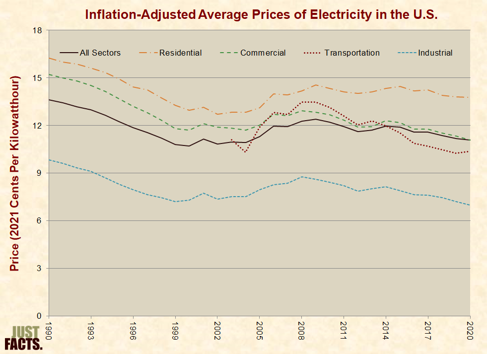
From 1929 to 1967, the inflation-adjusted average price of electricity for U.S. residential customers declined from about 60 cents per kilowatt hour to 10 cents, and it stayed roughly around this figure through 2012.[159]
* The inflation-adjusted average prices of electricity since 2004 for all U.S. consumers and the four major energy sectors are shown in the graph below:

Inflation-Adjusted Average Prices of Electricity in the U.S.

[160]

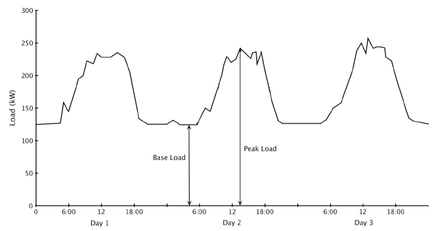
* Demand for electricity varies on an hourly, daily, and seasonal basis due to factors such as:

  • The time of the day, which influences the usage of lighting, computers, and other electric devices.
  • The weather, which influences the usage of heating, air conditioning, and ventilation systems.[161] [162] [163]

* As shown in the following graph, the terms “baseload” and “peak load” are used to describe the minimum and maximum demands for electricity over a given time period. The term “intermediate load” is used to describe the range between them.[164] [165]

Electricity Load Curve Example

[166]

  • Coal is the dominant energy source for generating baseload capacity, because low fuel costs make coal plants inexpensive to run continuously, which is ideal for generating baseload capacity. For the same reason, nuclear power is a primary source of baseload capacity. Natural gas, hydropower, geothermal, and waste-to-energy plants are also sources of baseload capacity.[167] [168] [169] [170]
  • Natural gas is the dominant energy source for generating intermediate and peak load capacity because natural gas power plants can ramp up and down quickly, which is ideal for intermediate and peak load capacity.[171] [172] [173] [174]
  • In 2009, natural gas became competitive with coal for generating baseload capacity in some areas of the U.S. This was primarily due to increased domestic natural gas production, which reduced prices. Other factors included increased coal prices, stricter environmental regulations, and expansion of natural gas pipelines.[175] [176] [177] [178]
  • In 2012, both coal and natural gas fuels were competitive for generating baseload capacity under differing circumstances in different regions of the U.S.[179]
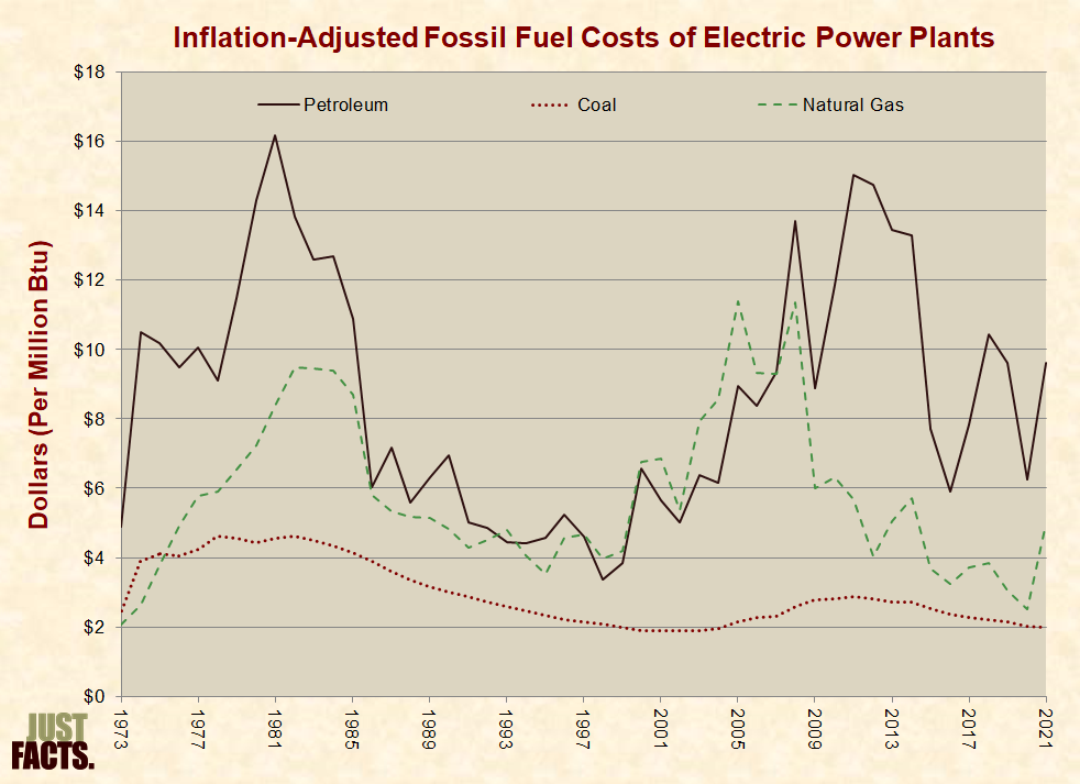
  • For existing power plants, natural gas plants that employ a high efficiency technology called “combined cycle” can generate baseload power less expensively than coal plants when natural gas is about 1.5 times the price of coal.[180] [181] [182] In 2015, the average energy-equivalent price paid by electric power plants for natural gas was about 1.5 times the price of coal.[183]
Inflation-Adjusted Fossil Fuel Costs of Electric Power Plants

[184] [185]

  • Per the U.S. Energy Information Administration (EIA), electric utilities and government entities that regulate them:

Forecast the demand for electricity at the time of the peak, and then identify existing and potential generating resources needed to satisfy that demand, plus enough additional resources to provide a comfortable reserve margin. The goal is to minimize the costs associated with new capacity investments while ensuring reliability for customers.[186] [187] [188]
Determining which electricity-generating technologies will provide the lowest cost while maintaining reliability is complicated by the following factors:

  • Power plants are capital-intensive and have lifespans measured in decades. Because these are long-term investments, there is ample time for market conditions and government energy polices to change, and this creates risk.[189] [190] [191] [192] [193] [194]
  • Utilities must produce enough electricity to meet their customers’ demands on a second-by-second basis, and the costs of generating this electricity vary depending upon when it is produced. During periods of high demand, electricity is more expensive to generate. Thus, technologies that generate electricity on demand have more value to utilities than intermittent resources, such as wind and solar.[195] [196] [197] [198] [199] [200] [201]
  • Decisions to invest in new generating capacity frequently involve factors that are unique to each utility and each point in time.[202]

* A commonly cited measure of the costs of building and operating new power plants is the “levelized cost” data published by EIA. Levelized costs reflect “both the capital and operating costs of deploying and running new utility-scale generation capacity of any given type.”[203] [204] Per EIA:

  • The direct comparison of LCOE [levelized cost of electricity] across technologies to determine the economic competitiveness of various generation alternatives is problematic and potentially misleading.”[205] [206]
  • The following features, caveats, and limitations are inherent in EIA’s levelized costs:
  • They remove the effects of government subsidies.[207]
  • They account for the costs of buying or leasing land to operate the generation facilities.[208]
  • They do not remove the effects of taxes or government regulations.[209] [210]
  • They do not measure actual costs but are projections of future costs.[211]

They vary with EIA’s assumptions:

    • In 2011, EIA reduced the projected 2016 levelized cost for wind by 35% below its projection from one year earlier.
      • In the same projections, EIA reduced the cost for photovoltaic (PV) solar by 47%.[212]
      • In 2015, EIA reduced the projected 2020 levelized capital cost for geothermal by 57% below its estimate from two years earlier.[213] [214]
  • They do not provide a comprehensive projection of future costs, because they estimate the cost of building and operating one new power plant of each technology. Beyond that, the prices of geothermal, wind, and hydropower are subject to change.[215]
  • EIA does not have a monitoring and feedback mechanism to test the accuracy of previous projections.[216]
  • The projections do not account for the fact that intermittent electricity is less valuable than electricity that can be dispatched on demand. Per EIA, the levelized costs for wind and solar “are not directly comparable to those for other technologies” and are therefore “listed separately in the tables, because caution should be used when comparing them to one another.”[217] [218] [219]
  • They do not account for the physical lifespan of different capital investments. Instead, they assume that all types of generation capacity have the same financial life (30 years).[220] [221] Differing technologies have different physical lifespans:
    • The majority of nuclear power plants have been licensed to operate for 60 years.[222]
    • Per a 2008 Congressional Budget Office report, “numerous power stations built in the first half of the previous century are still in use.”[223] [224]
    • Per a 2013 report commissioned by EIA, solar panels have an expected life of 20-30 years.[225]
  • They add a 3-percentage premium to the financing costs of coal power plants to account for risks that government may tax or regulate greenhouse gases.[226] In 2013, this increased EIA’s projected 2018 levelized cost for coal by 19%.[227]
  • They do not compare the costs of replacing existing capacity with new capacity. Unless the costs of building and operating new capacity are lower than the costs of operating existing capacity, there is an economic disincentive to displace existing plants.[228] [229]
  • They only analyze utility-scale systems.[230] Rooftop solar systems, which are typically installed on homes and commercial buildings, are more expensive than utility-scale systems. This is because utility-scale systems benefit from economies of scale.[231] [232]

In 2015, EIA projected the following levelized costs for plants that begin generating electricity in 2020:

Plant type (lowest cost option from each major category)

Cost (2013$/megawatthour)

Cost Increase Relative to Natural Gas

Dispatchable Technologies

Natural Gas Advanced Combined Cycle

72.6

0%

Geothermal

47.8

-34%

Conventional Coal

95.1

31%

Advanced Nuclear

95.2

31%

Non-Dispatchable Technologies

Onshore Wind

73.6

1%

Hydropower

83.5

15%

PV Solar

125.3

73%

[233]

* Per EIA, “a better assessment of economic competitiveness can be gained through consideration of avoided cost, a measure of what it would cost the grid to generate the electricity that is otherwise displaced by a new generation project, as well as its levelized cost.” Calculating these costs involves a greater degree of complication than levelized costs.[234] [235]
* In July 2013, EIA published a preliminary discussion paper using avoided costs and levelized costs to compare the projected 2018 and 2035 values of advanced combined cycle natural gas (Adv CC), onshore wind, and PV solar with different subsidies given to wind and solar.[236] Because there is significant variability in factors that affect electricity costs and values in different regions of the country, the paper contained assessments of 22 regions within the U.S. electricity system. It found that without subsidies for wind and with a 10% investment tax credit for solar:

  • In 2018, the projected economic value of the wind and solar systems is “negative and significantly below” natural gas advanced combined cycle projects “in all regions.”
  • By 2035, the economic value of onshore wind is positive in 6 of 20 regions where the technology can be built, and in 3 of 21 regions for solar PV (with 5 additional regions close to breakeven).”
  • “Direct comparison of LCOE values significantly understate the advantage of Adv CC relative to onshore wind in terms of economic value in all regions, while overstating the advantage of Adv CC relative to solar PV….”
  • “Solar LCOE remains substantially higher than wind LCOE throughout the projection period….”[237]

* The following features, caveats, and limitations are inherent in this analysis:

  • It is based on projections of changing future economic conditions, such as rising natural gas prices starting around 2025.[238] [239]
  • It does not provide an analysis of solar without the effect of government subsidies.[240]
  • It does not remove the effects of existing taxes or government regulations.[241] [242]

It does not provide a comprehensive projection of future costs, because it estimates the cost of building and operating one new power plant of each technology. Beyond that, the prices of geothermal, wind, and hydropower are subject to change.[243]

  • It does not account for the physical lifespan of different capital investments. Instead, it assumes that all types of generation capacity have the same financial life (30 years).[244]
  • It only analyzes utility-scale systems.[245] Rooftop solar systems, which are typically installed on homes and commercial buildings, are more expensive than utility-scale systems. This is because utility-scale systems are larger and benefit from economies of scale.[246] [247]

* In 2015, EIA used levelized costs and avoided costs to estimate which type of plants would be economically competitive to build and begin producing electricity in 2020. Positive values indicate an economic incentive to build, and negative values indicate a disincentive:[248]

Plant type (lowest cost option from each major category)

Incentive (Levelized Minus Avoided Costs)

Incentive Relative to Natural Gas

Dispatchable Technologies

Natural Gas Advanced Combined Cycle

-1

0

Geothermal

27

28

Conventional Coal

-24

-23

Advanced Nuclear

-23

-22

Non-Dispatchable Technologies

Onshore Wind

-9

-8

Hydropower

-14

-13

PV Solar

-34

-33

[249]

  • Forest product companies often use byproducts from their operations to generate their own electricity.[250] During 2015, wood generated 1.0% of all electricity in the U.S., as compared to 0.9% for solar and 0.4% for geothermal.[251]
  • Oil and biofuels are rarely used to create electricity, because they are significantly more costly than the major sources of electricity.[252] [253] In 2015, the average energy-equivalent price paid by electric power plants for petroleum was about 3.1 times the price of coal.[254]

Petroleum

    • Petroleum is a class of fossil fuels that are generally liquid at atmospheric pressure, although broader definitions of the term also include some gases and solids. The terms “petroleum” and “crude oil” are sometimes used synonymously, although petroleum is typically defined to include several other types of fossil fuels.[255] [256]
    • Petroleum is primarily comprised of organic compounds called hydrocarbons, which consist of carbon and hydrogen. Other common elements of petroleum are nitrogen, oxygen, and sulfur.[257] [258] [259]
    • Petroleum is mainly thought to be formed of diverse marine organisms that were buried by sediments and transformed by heat, pressure, and time.[260] [261] [262]

    The first oil well was drilled in 1857, the first intercontinental oil shipment occurred in 1859, and the first modern oil refinery commenced operations in 1862. By the 1870s, “refineries, tank cars, and pipelines had become characteristic features of the industry,” and by 1874, U.S. crude oil production had grown to 10 million barrels per year.[263]
    Today, the vast majority of crude oil is transported via pipelines and ships, and most refined petroleum fuels are transported from refineries to wholesale terminals through pipelines. Pipelines are the safest and most economical means of transporting petroleum in the U.S.[264] [265] [266] [267] [268]
    Petroleum is used to manufacture wide-ranging products, such as gasoline, diesel fuel, jet fuel, heating oil, lubricants, asphalt, propane, synthetic fabrics, plastics, paints, fertilizers, and soaps.[269] [270]

  • In 2015, petroleum supplied:
  • 35% of all primary energy consumed in the U.S.
  • 92% of primary energy consumed in the transportation sector.
    • 39% of primary energy consumed in the industrial sector (not including energy purchased from electric power utilities).
    • 15% of primary energy consumed in the residential and commercial sectors (not including energy purchased from electric power utilities).
    • 1% of primary energy consumed in the electric power sector.[271]

    Consumption, Production, Imports, and Prices

    • In 2015, the U.S. consumed about 6.7 billion gallons of petroleum, 25% of which was imported.[272]
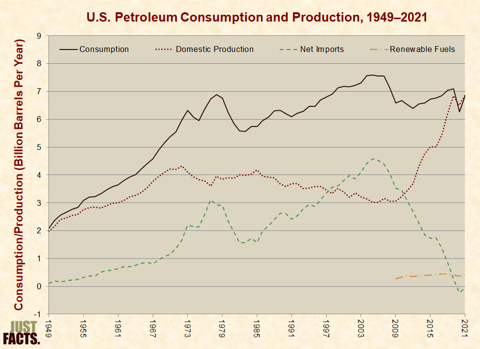
    • U.S. petroleum consumption and net imports have declined since the mid-2000s, primarily due to the economic recession, increases in domestic crude oil production, use of renewable fuels, and efficiency improvements:[273] [274]
    Petroleum Consumption and Production

    [275]

    • In 2014, U.S. net petroleum imports were distributed as follows:
    • 61% came from countries in the Western Hemisphere and 37% from the Persian Gulf.[276]
    • Among the top five countries, 51% came from Canada, 23% from Saudi Arabia, 14% from Venezuela, 7% from Iraq, and 6% from Russia.[2 77]
    • 59% came from nations that are members of the Organization of the Petroleum Exporting Countries (OPEC),[278]
    • An intergovernmental body formed to “coordinate and unify the petroleum policies of its member countries.”[279] OPEC members include: Algeria, Angola, Ecuador, Indonesia, Iran, Iraq, Kuwait, Libya, Nigeria, Qatar, Saudi Arabia, United Arab Emirates, and Venezuela.[280]

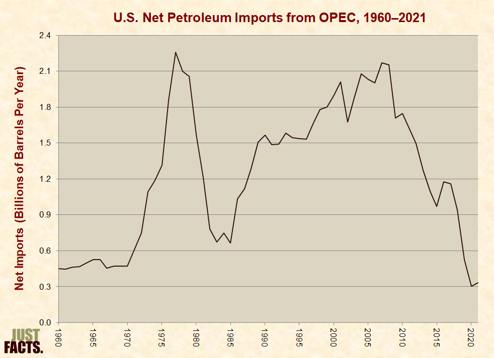
    * Since OPEC’s founding in 1960, its member nations have adopted various strategies to exert control over the petroleum market. One of their more common strategies has been to limit their petroleum production in order to boost prices and increase their profits.[281] [282] [283]
    * OPEC nations have also adopted the opposite strategy of maximizing their petroleum production in order to drive down prices, force their competitors out of business, and grow their market share. Some OPEC nations have recently done this in response to increased production from non-OPEC countries.[284] [285] [286] [287] [288] [289]

    US Imports from OPEC

    [290]

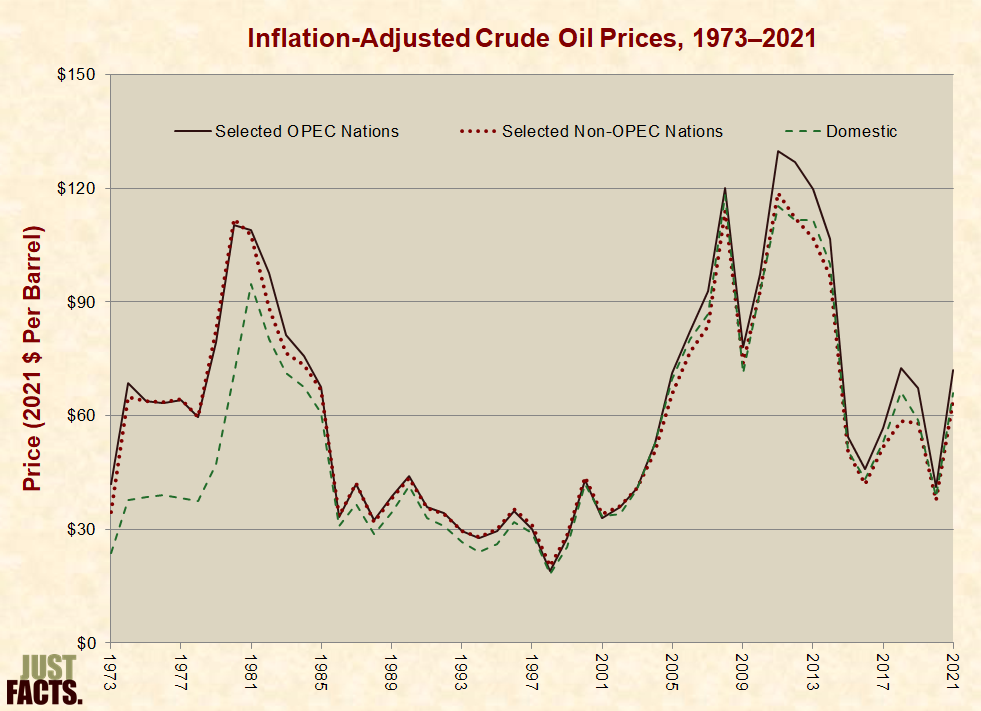
    * Crude oil prices are affected by global and local factors that impact the supply of petroleum and the demand for petroleum products, such as economic growth and recessions, OPEC policies, political unrest, and technological advancements.[291] [292] [293] [294]

    Inflation-Adjusted Crude Oil Prices

    [295]

    * In the U.S. during 2015, the average landed (i.e., delivered) price of crude oil from selected OPEC nations was 8% more than the average price of domestic crude, and the average landed price of crude from selected non-OPEC nations was 1% less than the average price of domestic crude.[296]
    * In 2015, the average retail price of a gallon of regular-grade gasoline in the U.S. was $2.42. Crude oil accounted for 48% of this price, refining costs and profits accounted for 19%, federal and state taxes accounted for 19%, and distribution and marketing accounted for 14%.[297]


    Extraction Methods

    * Crude oil resources[298] can be grouped into four major categories based upon their accessibility:

        1. conventional oil, which is located in porous rocks and reservoirs that allow the oil to freely flow to the surface of the earth when it is accessed through drilling.[299] [300]
        1. tight oil (sometimes called shale oil[301] [302] [303]), which is located in semi-porous or non-porous rocks that don’t allow the oil to freely flow when accessed through drilling. This type of petroleum can be extracted by using a combination of technologies known as horizontal drilling and hydraulic fracturing (described below).[304] [305] [306]
        1. oil sands (sometimes called tar sands), which are comprised of clay, sand, water, and a thick oil known as bitumen. Bitumen it too thick to pump from the ground, and thus, oil sands are generally mined and then the bitumen is extracted.[307] [308]
        1. oil shale (note the difference in word order from shale oil), which is rock containing solid hydrocarbons that become liquid and can be extracted after being heated to 650-1,000 degrees Fahrenheit. At the moment, it is not profitable to extract petroleum from oil shale.[309] [310] [311] [312]

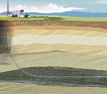
    * Horizontal drilling involves penetrating the ground vertically (like traditional drilling) and then turning horizontally in order to drill along the layer that contains the fossil fuel resources. This method of drilling exposes more of the fossil fuel resources to the bore of each well, thus increasing yields, decreasing the surface footprint of drilling operations, and decreasing unwanted output from the wells, such as water.[313] [314]

    Horizontal Drilling

    [315]

    * Horizontal drilling was first successfully employed in 1929 and has been used commercially since the late 1980s. By 1990, more than 1,000 horizontal wells were drilled worldwide, roughly 85% of which were in Texas.[316]
    * Hydraulic fracturing or fracking involves injecting fluids at high pressures from the bore of the well into the layer that contains the fossil fuel resources. This process creates fractures in the rock, which allows oil to flow to the bore of the well. The fluids used for fracking typically contain sand or ceramic beads that serve to hold open the fractures after they have been created. This fluid also contains varying chemicals that are used for purposes such as reducing friction and preventing pipe corrosion.[317] [318] [319] (A detailed description of the process is shown in the video below.)
    * Hydraulic fracturing was first successfully employed in 1947 and has been used commercially since the 1950s. By 1955, more than 100,000 fracking treatments were performed.[320]
    * Since the mid-2000s, technological advancements and market conditions have made it economically worthwhile to extract tight oil by using a combination of horizontal drilling and hydraulic fracturing.[321] [322] [323] [324] [325] [326] The process is shown in this video:

    * From 2005 to 2015, U.S. crude oil production increased by 65%, primarily due to the use of horizontal drilling coupled with hydraulic fracturing in tight oil formations.[327] [328] [329] [330] [331] [332]
    * As of 2015, horizontal drilling coupled with hydraulic fracturing had not been widely used to extract tight oil outside the U.S.[333] [334] [335] [336] [337] In 2013, the U.S. Energy Information Administration (EIA) estimated that 10% of worldwide technically recoverable oil resources are located in tight formations.[338]
    * For facts about the environmental impacts of horizontal drilling and hydraulic fracturing, visit the politics section of this research.
     

    ….To be continued…

    Email this author

Posted in Energy | Comments Off on Energy Facts and Figures Part III